Home Grown Spectrum Waterfalls
Introduction to RTSA & Python Integration
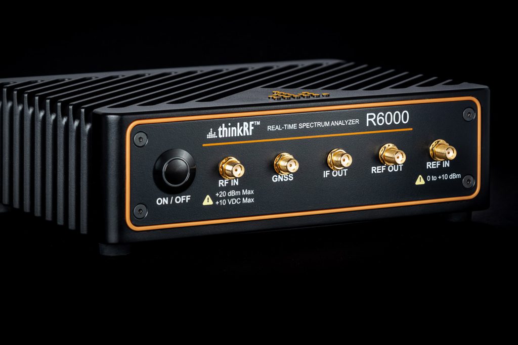
Real-Time Spectrum Analyzers (RTSAs) capture and analyze the frequency spectrum in real time. thinkRF’s RTSAs offer advanced features for applications like spectrum monitoring and signal intelligence, providing high-fidelity IQ data crucial for detailed analysis of complex signal environments. However, finding an exact application for a specific need can be challenging. Homegrown solutions often work best. thinkRF’s API supports Python and C++, simplifying custom application creation.
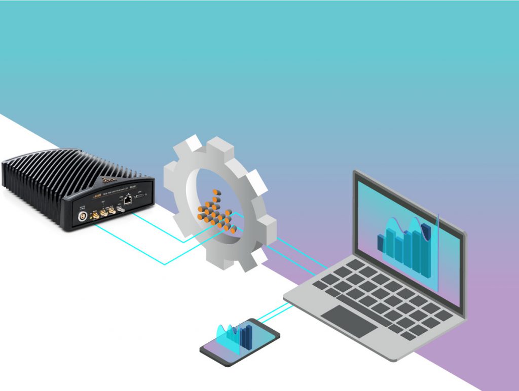
Integrating thinkRF RTSAs with Python, benefits researchers and startups who require to perform specific analysis or insights. Python’s simplicity and extensive libraries make it ideal for developing custom RF analysis applications. thinkRF’s PyRF framework simplifies interfacing with thinkRF devices, easing data acquisition, signal processing, and enabling rapid development and innovation. Thus, capturing, processing, and visualizing data programmatically leads to powerful applications with deeper insights into signal and spectrum analysis.
This blog will guide you through capturing IQ data from a thinkRF RTSA and creating a 3D waterfall plot using Python, demonstrating the ease and excitement of developing code for RTSA interaction.
Setting Up the Python/PyRF Environment
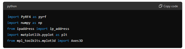
Before diving into the code, let’s set up the necessary Python environment. Ensure you have Python installed on your system. You’ll also need the following packages:
- PyRF4 (for interfacing with thinkRF devices)
- NumPy (for numerical operations)
- Matplotlib (for plotting)
Details can be found on thinkRF’s API Page
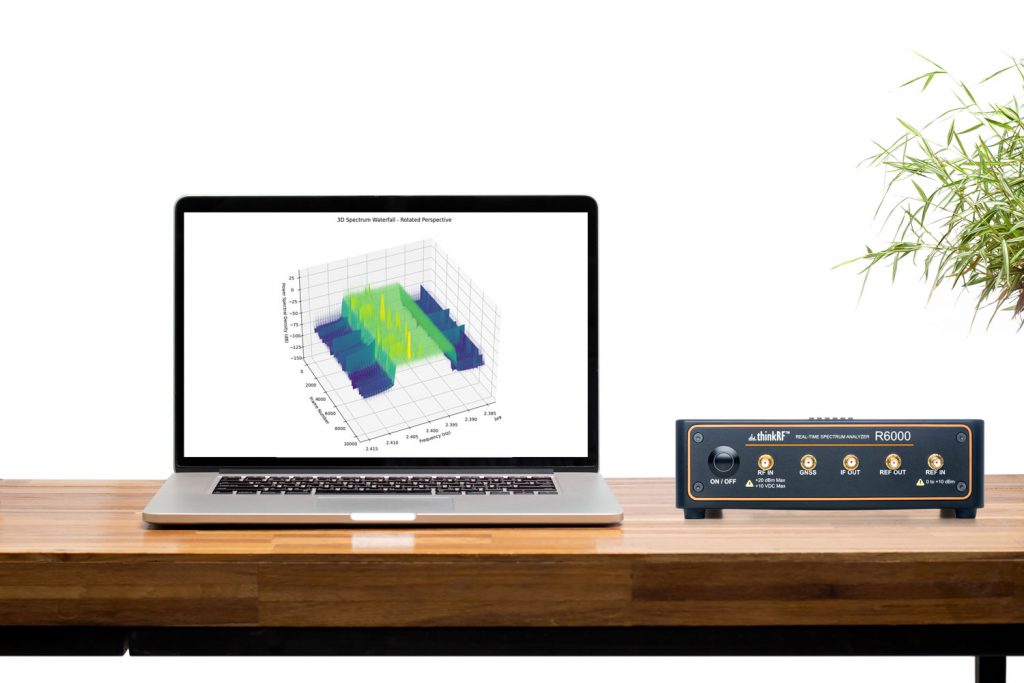
3D Spectrum Waterfall Plots
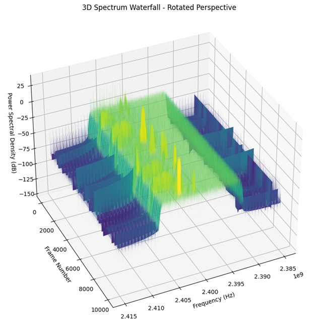
A 3D Spectrum Waterfall Graph is a visualization tool in spectrum analysis that displays the power spectral density of a signal over time. It combines three dimensions: frequency, time, and power level, to provide a detailed view of the signal environment. The graph shows frequency on one axis, time on another, and power level as a color or height, creating a dynamic representation of the signal’s spectral characteristics.
3D Waterfall Plots are incredibly helpful in the field of spectrum analysis because they provide a dynamic, three-dimensional view of how the power spectral density of a signal varies over time. This comprehensive visualization allows for a deeper understanding of the spectral content, offering insights that are not immediately obvious in traditional two-dimensional plots. The three-dimensional aspect of the plot makes it easier to observe changes and trends. For instance, it’s easier to spot a frequency hopping signal in a waterfall relative to a two-dimensional FFT view.
By incorporating time as a dimension, 3D plots reveal how spectral characteristics evolve. This is crucial for monitoring changes, detecting intermittent interference, and understanding periodic patterns. Viewing frequency, time, and power levels simultaneously provides a comprehensive view of the signal environment, essential for signal intelligence and spectrum management.
Patterns and anomalies are more apparent in 3D, aiding quick and accurate signal identification. In real-time applications, 3D waterfall plots offer continuous, immediate insights, enabling proactive responses.
Let’s get to coding!
Now, let’s dive into the code that captures IQ data from the thinkRF RTSA and creates a 3D waterfall plot.
First, import the necessary packages:
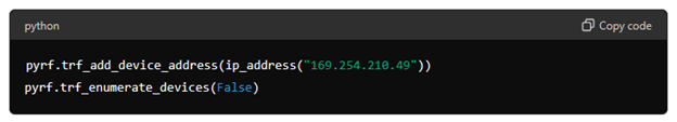
Next, add the device’s IP address and enumerate the device:
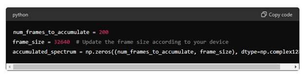
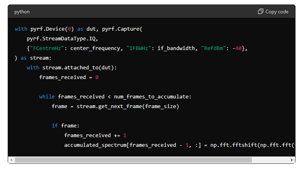
We then set up the parameters for capturing IQ data. Define the number of frames to accumulate and initialize an array to store the spectra:
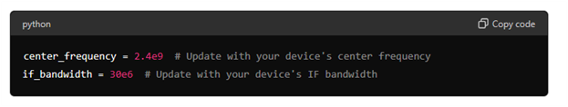
Set the center frequency and IF bandwidth based on your device specifications:
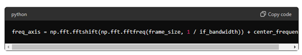
Calculate the frequency axis based on the center frequency and IF bandwidth:
Connect to the device and create a capture stream with the specified parameters:
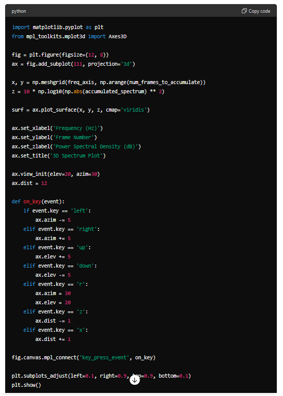
We visualize the accumulated spectrum data using a 3D plot. The Matplotlib library allows us to create a 3D surface plot, where the x-axis represents frequency, the y-axis represents frame numbers, and the z-axis represents power spectral density in dBm.
Empower Your thinkRF RTSA with Python
By capturing IQ data from a thinkRF RTSA and visualizing it with a 3D waterfall plot, you can gain comprehensive insights into the spectral environment, making it an invaluable tool for both practical applications and advanced research. In the next blog, we will walk through the Python code to capture IQ data from a thinkRF RTSA and create a 3D waterfall plot, demonstrating how you can leverage this powerful visualization tool in your own projects.
Stay tuned for more tuned for more “Empower Your thinkRF RTSA with Python” ideas and insights!